Quickstart AltaiPony: De-trend and find flares
AltaiPony works off of the lightkurve package, with a
FlareLightCurve being a subclass of the more general LightCurve.
So, to get started with AltaiPony, you first want to get a light
curve via lightkurve.
import lightkurve as lk

from altaipony.customdetrend import custom_detrending
from altaipony.lcio import to_flare_lightcurve

import matplotlib.pyplot as plt
Let’s start by searching for AU Mic, a young, active star, observed with
TESS with search_lightkurve. (Consult the docs of lightkurve for
the various parameters.)
# get a table of light curves from MAST
lc_table = lk.search_lightcurve('AU Mic', mission='TESS', author='SPOC')

lc_table
# |
Mission |
Year |
Author |
Exptime (s) |
Target Name |
Distance (arcsec) |
|---|---|---|---|---|---|---|
0 |
TESS Sector 01 |
2018 |
SPOC |
120 |
441420236 |
0.0 |
1 |
TESS Sector 27 |
2020 |
SPOC |
20 |
441420236 |
0.0 |
2 |
TESS Sector 27 |
2020 |
SPOC |
120 |
441420236 |
0.0 |
3 |
TESS Sector 95 |
2025 |
SPOC |
20 |
441420236 |
0.0 |
4 |
TESS Sector 95 |
2025 |
SPOC |
120 |
441420236 |
0.0 |
Let take the first on the list, download it and plot it:
%matplotlib inline
lc = lc_table[0].download()
lc.plot();
5% (982/19261) of the cadences will be ignored due to the quality mask (quality_bitmask=175).
5% (982/19261) of the cadences will be ignored due to the quality mask (quality_bitmask=175).

We can immediately see that there are some flares (bursty positive
excursions). Now let’s make lc a FlareLightCurve object using the
to_flarelightcurve function:
flc = to_flare_lightcurve(lc)
flc.plot();

Note that this preserves the functions that you are used to from
lightcurve, such as plot(). Nifty.
Let’s check what’s changed:
flc
FlareLightCurve(ID: 441420236 | Mission: TESS | QCS: 1 | Cadence: 120 s
The above tells us that we have indeed created a FlareLightCurve,
and it still has all the attributes, plus some more, like an empty flare
table, and an empty detrended flux column.
This is the raw light curve. The is intrumental noise but also stellar
variability. Let’s remove it with the custom_detrending function:
flcd = flc.detrend("custom", func=custom_detrending, spline_coarseness=8)

plt.figure(figsize=(10, 5))
plt.plot(flc.time.value, flc.flux, label='Original Flux', alpha=0.5)

plt.plot(flcd.time.value, flcd.detrended_flux, label='Detrended Flux', color='orange')
plt.xlabel('Time')
plt.ylabel('Flux')
plt.title('Custom Detrending of Flare Light Curve')
plt.legend();

custom_detrending runs a spline fit and two rounds of Savitzky-Golay filtering with decreasing windows, while iteratively masking outliers that could be flare candidates to find a model light curve, and subtract it from the observed one.
flcd = flcd.find_flares()
flcd.flares.sort_values(by="ed_rec", ascending=False)
Found 41 candidate(s) in the (0,8949) gap.
Found 28 candidate(s) in the (8949,14785) gap.
Found 3 candidate(s) in the (14785,14973) gap.
Found 12 candidate(s) in the (14973,17693) gap.
Index |
istart |
istop |
cstart |
cstop |
tstart |
tstop |
ed_rec |
ed_rec_err |
ampl_rec |
dur |
n_valid |
|---|---|---|---|---|---|---|---|---|---|---|---|
72 |
14974 |
15060 |
87456 |
87732 |
1348.927 |
1349.311 |
802.47 |
0.707 |
0.03181 |
0.383 |
17693 |
68 |
14631 |
14784 |
86616 |
86794 |
1347.761 |
1348.008 |
581.10 |
0.357 |
0.02975 |
0.247 |
17693 |
30 |
6517 |
6634 |
77508 |
77625 |
1335.111 |
1335.274 |
93.41 |
0.183 |
0.03255 |
0.162 |
17693 |
65 |
14426 |
14604 |
86350 |
86568 |
1347.391 |
1347.694 |
57.61 |
0.389 |
0.00548 |
0.303 |
17693 |
0 |
521 |
614 |
71430 |
71525 |
1326.669 |
1326.801 |
46.93 |
0.207 |
0.01085 |
0.132 |
17693 |
… |
… |
… |
… |
… |
… |
… |
… |
… |
… |
… |
… |
35 |
7536 |
7539 |
78537 |
78540 |
1336.540 |
1336.544 |
0.304 |
0.042 |
0.00110 |
0.004 |
17693 |
61 |
14233 |
14236 |
86142 |
86145 |
1347.102 |
1347.107 |
0.295 |
0.043 |
0.00089 |
0.004 |
17693 |
6 |
1450 |
1453 |
72374 |
72377 |
1327.981 |
1327.985 |
0.284 |
0.043 |
0.00096 |
0.004 |
17693 |
78 |
15921 |
15924 |
88623 |
88626 |
1350.548 |
1350.552 |
0.280 |
0.043 |
0.00092 |
0.004 |
17693 |
55 |
13337 |
13340 |
85232 |
85235 |
1345.839 |
1345.843 |
0.262 |
0.043 |
0.00087 |
0.004 |
17693 |
The individual columns show:
istart/istop: Start/stop indices in the original flux array
cstart/cstop: Start/stop indices in the cadence array
tstart/tstop: Start/stop times in BKJD or BTJD
ed_rec: Recovered equivalent duration (ED)
ed_rec_err: Error in recovered ED
ampl_rec: Recovered amplitude in relative flux units
dur: Duration of flare in days
n_valid: Total number of valid data points in light curve
Now, let’s keep only some 3 medium-sized flares to showcase fitting
flcd.flares = flcd.flares.iloc[10:13]
flcd.flares
Index |
istart |
istop |
cstart |
cstop |
tstart |
tstop |
ed_rec |
ed_rec_err |
ampl_rec |
dur |
n_valid |
|---|---|---|---|---|---|---|---|---|---|---|---|
10 |
1993 |
2001 |
72918 |
72926 |
1328.736 |
1328.747 |
2.13 |
0.057 |
0.00631 |
0.011 |
17693 |
11 |
2410 |
2417 |
73340 |
73347 |
1329.322 |
1329.332 |
1.35 |
0.064 |
0.00248 |
0.010 |
17693 |
12 |
2451 |
2465 |
73381 |
73396 |
1329.379 |
1329.400 |
5.19 |
0.077 |
0.00771 |
0.021 |
17693 |
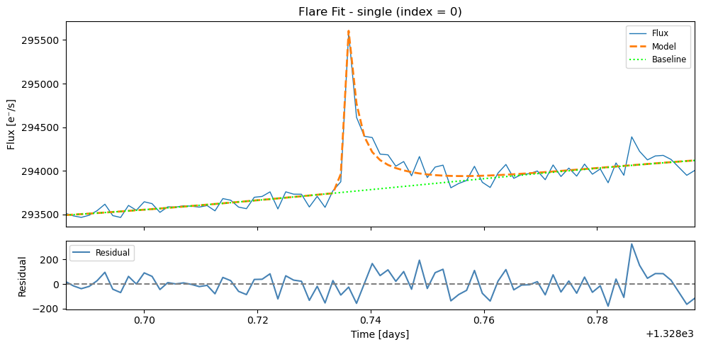
This flare table gives a first impression of where the flares are found,
and what their properties are. To get a better estimate, you can fit a
flare template to each detection using fit_flares(), which follows
the procedure described in Guenther et
al. (2020):
flcd.fit_flares(max_flares=3, plot=True, n_steps=1500, discard=100)
Fitting region from 1328.68612 to 1328.79723; Region [0](max. number of flares in group = 3 x 1)
100%|██████████| 1500/1500 [00:42<00:00, 35.19it/s]
100%|██████████| 1500/1500 [00:38<00:00, 39.27it/s]
Fitting region from 1329.27222 to 1329.45000; Region [1](max. number of flares in group = 3 x 2)
100%|██████████| 1500/1500 [00:47<00:00, 31.43it/s]
100%|██████████| 1500/1500 [00:50<00:00, 29.55it/s]
100%|██████████| 1500/1500 [00:55<00:00, 26.90it/s]
100%|██████████| 1500/1500 [00:51<00:00, 29.27it/s]
100%|██████████| 1500/1500 [00:52<00:00, 28.52it/s]
100%|██████████| 1500/1500 [00:56<00:00, 26.60it/s]
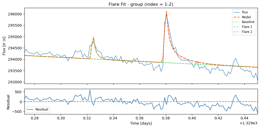
flcd.flare_table()
Index |
t_peak |
t_peak_err |
fwhm |
fwhm_err |
amplitude |
amplitude_err |
ed_rec |
fit_type |
group_index |
|---|---|---|---|---|---|---|---|---|---|
0 |
1328.736142 |
0.000082 |
0.004722 |
0.000472 |
1882.62 |
103.32 |
2.50 |
single |
– |
1 |
1329.323987 |
0.000098 |
0.001450 |
0.000970 |
3420.59 |
3200.51 |
1.05 |
group_member |
1 |
2 |
1329.379935 |
0.000131 |
0.006053 |
0.001044 |
2899.35 |
870.77 |
4.65 |
group_member |
1 |
Note that the columns in this flare_table are different from the flares table:
t_peak: Time of flare peak in BKJD or BTJD
t_peak_err: Error in flare peak time
fwhm: Full Width at Half Maximum of the flare profile (days) – Davenport+2014 model
fwhm_err: Error in FWHM measurement
amplitude: Peak amplitude of the flare in flux units
amplitude_err: Error in amplitude measurement
ed_rec: equivalent duration (ED) of the fitted model
fit_type: Type of fit applied (single flare or group member)
group_index: Group identifier for clustered flares (empty for single flares)
For a deeper dive into the flare finding pipeline, see the Flare Fitting tutorial